

How do I throw high scoring darts?
Analysing the standard dartboard
This post draws on methods outlined in the paper A Statistician Plays Darts, by Ryan J. Tibshirani, Andrew Price and Jonathan Taylor. I will refer to the paper as ASPD for the rest of the post.
Consider a player (Alice) throwing darts at the standard dart board. In a normal game (or leg in a professional match), Alice starts with a total score of 501, and the score from each dart is taken off her total. Therefore, at least in the early stages of the game, she is seeking to maximise the score of each dart. A good player will obviously aim for the highest scoring regions of the board (the triple $20$, the bullseye, the triple $19$). However, this may not be a good strategy for an amateur player - for example, the triple $20$ region is surrounded by low scoring regions (e.g. in the $1$ and $5$ segments), meaning a minor miss could drastically affect her score. So Alice may be better off aiming at a lower scoring region, surrounded by regions of similar score, so as to minimise the risk of hitting these regions due to a less accurate aim.
How should we quantify Alice’s ability? To start with, let’s make the simplifying assumption that when she aims at a particular point on the dartboard $p$, the probability of the dart hitting the board at a specific location $Z$ is given by a 2-D spherical Gaussian distribution:
\[Z\sim N(p, \sigma^2 \mathbf{I})\]The parameter $\sigma$ is the standard deviation parameter of the throw, and parameterises the skill level of the player. This is the initial assumption made in ASPD; later, we will follow the lead of ASPD in generalising this to a general covariance matrix $\Sigma$.
$Z$ is a random variable, taking values in $\mathbb{R}\times\mathbb{R}$; the score of the dart is a function $s:Z\mapsto s(Z)\in \mathbb{N}_0$, returning the score of the region of the dartboard that the dart hit. This is what the scoring function looks like, applied to each region of the dartboard:
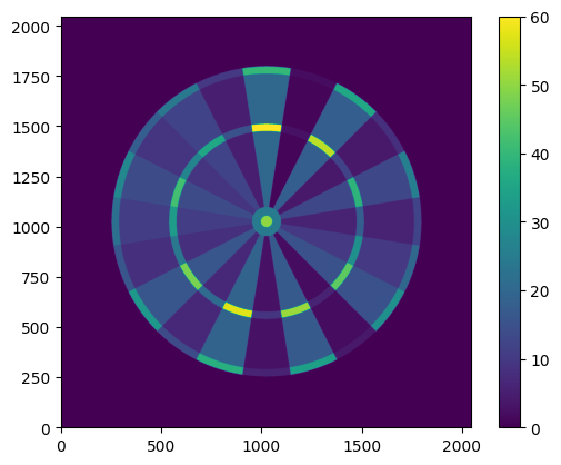 |
|---|
| Heatmap of scores for the conventional dartboard |
Suppose that Alice aims at a point $p$ on the board, with throwing distribution $Z\sim N(p, \sigma^2 \mathbf{I})$. The key insight of ASPD is that the expected score of the dart is given by a convolution of a Gaussian probability density function (pdf) and the scoring function $s$:
\[\begin{align} \mathbf{E}_{p,\sigma}\left[s(Z)\right] &= \int_{\mathbb{R}\times\mathbb{R}}f_{p,\sigma}(x, y)s(x, y)\;\mathrm{d}x\mathrm{d}y \\ &= \left(f_{0,\sigma}*s\right)(p) \end{align}\]where $f_{p,\sigma}$ is the probability density function of a 2-D Gaussian random variable with mean $p$ and covariance matrix $\sigma^2\mathbf{I}$. This convolution can be computed easily by taking advantage of the identity:
\[f*g = \mathcal{F}^{-1}\left[\mathcal{F}(f)\cdot\mathcal{F}(g)\right]\]where $\mathcal{F}(f)$ is the Fourier transform of the function $f$. This can be efficiently computed for all positions $p$ on the board, using the fast Fourier transform (FFT), an algorithm available out of the box from many scientific programming libraries such as numpy.
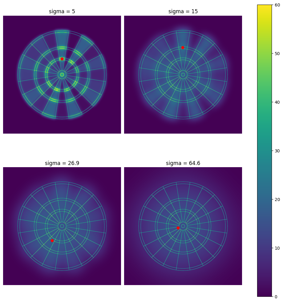
Let’s start be recreating some of the heat plots produced in ASPD, using a range of $\sigma$ values to represent players of different abilities. The temperature of the heat plot indicates the expected score obtained when aiming at that point; also marked is the maximum expected value, i.e. the point at which the player should aim to maximise the expected score.
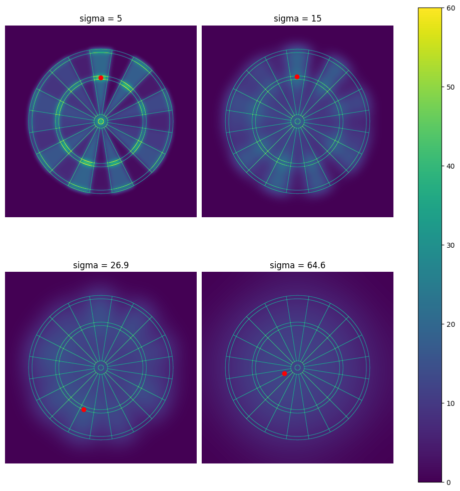 |
|---|
| Expected score heatmaps, for 4 values of $\sigma$, including two from the original ASPD paper. |
We see from these plots that strong players should aim for the triple $20$ to maximise their $1$-dart score. However, once the player’s skill level falls below a certain skill threshold, this switches over to the triple $19$. As the throwing distribution gets more and more spread (i.e. as $\sigma$ increases), the optimal aim spot moves closer to the bullseye. As the skill of the player decreases, the maximum expected score that the player can expect to achieve also decreases.
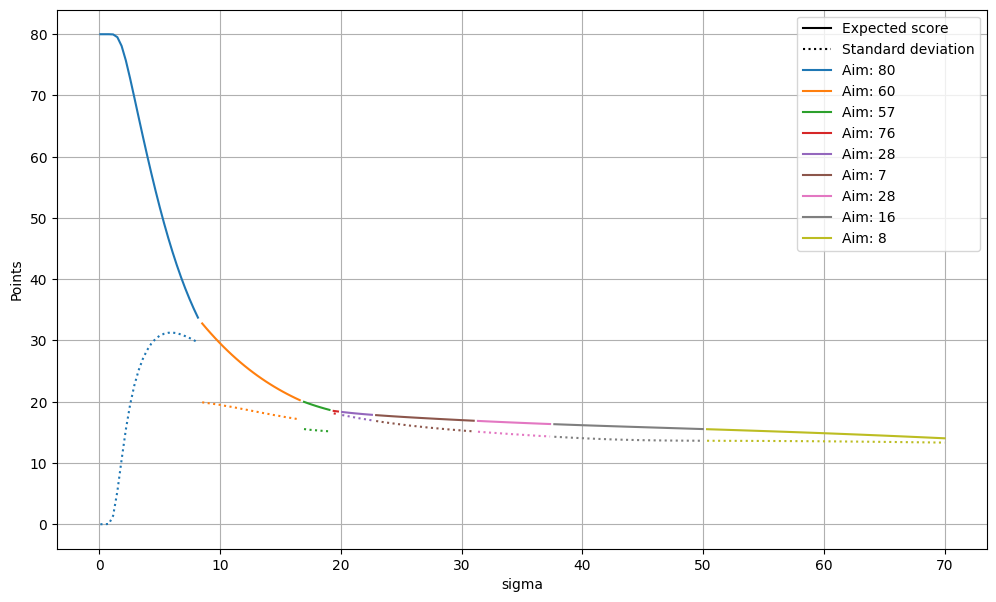
The visualizations above have been used to find the optimal aiming points for 4 specific values of $\sigma$. Instead, let’s look at a range of possible values, and identify the optimial aiming point, the maximum expected score, and the standard deviation of the score when aiming for this point:
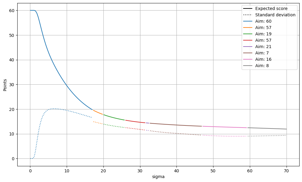 |
|---|
| Expected score and standard deviation as $\sigma$ increases from 0 up to 70mm. The colours represent the regions of the dartboard that are being aimed at, for each choice of $\sigma$. |
The takeaways from this plot are:
-
For players with $\sigma<17$ millimetres, the triple $20$ is the best place to aim. As $\sigma$ rises from $0$, the standard deviation of the expected score rises until it reaches a maximum at $\sigma=6.5$ millimetres, after which it begins to decrease. Expected scores decrease from the maximum of $60$ (for players with near perfect aim) down to $20$ as $\sigma$ increases.
-
At $\sigma\approx 17$ millimetres, the optimal aim point makes a discontinuous jump to the triple $19$. The exact aim point is not always in the triple $19$ region - for example, it drifts slightly outside the triple $19$ region into the single $19$ region, taking advantage of the larger surface area of the outer single $19$ region. Expected scores for players with this skill level are in the $15-20$ point range.
-
As $\sigma$ increases further, the optimal point drifts upwards and closer to the bullseye, to minimise the probability of missing the board entirely and scoring $0$. The expected score drops more slowly as $\sigma$ increases, staying above $10$ expected points even for large values of $\sigma$.
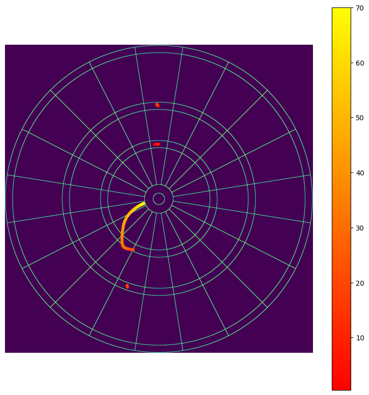
We can also visualize the path that the optimal point traces across the face of the dartboard, as $\sigma$ increases:
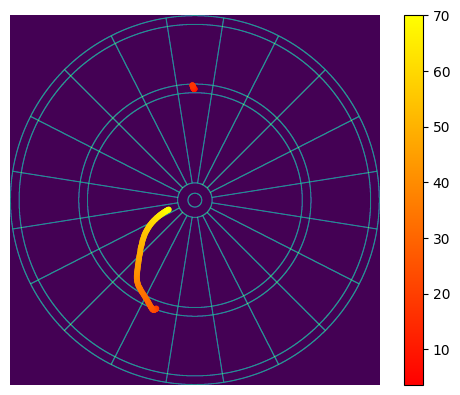 |
|---|
| The optimal path of aim points, moving across the board as $\sigma$ increases. |
The following video shows how the heat map of expected score changes as $\sigma$ increases - the frames are normalized so that the brightest colour corresponds to the current largest expected score. This makes the change in the heat map easier to see, and shows how the optimal aiming point moves up towards the bullseye in the limit of $\sigma\rightarrow\infty$.
General $\Sigma$
The analysis up until now has focussed entirely on a particular kind of throwing distribution - specifically, distributions which are spherically symmetric, and so parameterised by a single parameter $\sigma$:
\[\Sigma_{sph} = \sigma^{2}\mathrm{I}\]This has been convenient, as it means that the player’s skill is represented by the single parameter $\sigma$, making it easier to visualise performance as a function of skill. Of course, it is possible to model the player’s throwing distribution using a more general set of throwing distributions, by allowing $\Sigma$ to be any symmetric positive semi-definite matrix. In fact, as pointed out in ASPD, this is likely to be observed in the throwing distributions of real players:
- There is usually a larger variance in the vertical direction than the horizontal direction, as it is harder to account for the additional affect of gravity on the dart in this direction. So a more representative throwing distribution can be modelled using a diagonal covariance matrix with distinct horizontal and vertical variances:
-
A general covariance matrix $\Sigma$ with off-diagonal components may be needed to fully represent the throwing distribution of a player. For example, for a right-handed player, the angle that the forearm makes with the vertical when throwing dart may influence the accuracy in a direction no parallel to the vertical or horizontal axes. In fact, the authors of ASPD find exactly this when measuring their own personal observed throwing distributions (see Figure 4 in their paper).
-
The authors of ASPD also investigate alternative, non-Gaussian models which are able to capture effects such as skewness, not represented in the simplified Gaussian model. However, they find that the added complexity does not provide much additional value over the Gaussian model.
-
The assumption of a constant throwing distribution may also be too restrictive. There are ways in which one might expect the parameters of the distribution to change, both in space (e.g. when aiming at different parts of the board, such as a double) and in time (when the player has had a chance to ‘warm up’).
In the case of a general positive-definite symmetric covariance matrix $\Sigma$, we can visualize the heat map and recommended aiming point in the same way as before. For example, here is the heat map for the throwing distribution with non-diagonal covariance given by:
Sigma = np.array([[400, 500], [500, 900]]) # note: units here are pixels, not mm
As mentioned earlier, this has a larger variance in the vertical direction, and has a slight leftwards tilt corresponding to a right-handed player. We see that the triple $15$ is recommended now, due to the smaller variance in the direction in the direction perpendicular to the $15$ segment.
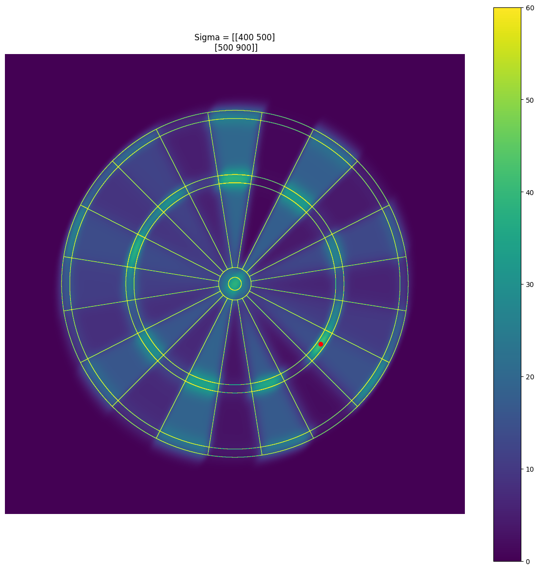 |
|---|
| Expected score heatmap for a more general throwing distribution. Note that the recommended aiming point is now in the lower right quadrant, reflecting the tilt of the throwing distribution. |
Aiming at the Quadro board
The analysis performed above can be applied just as well to the Quadro board - as a reminder, this board has an additional ring between the centre and the triple ring which quadruples the score of the segment:
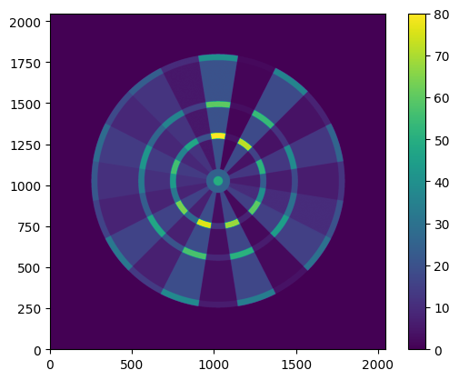 |
|---|
| Heatmap of scores for the Quadro dartboard |
For the same values of $\sigma$ plotted earlier, we can visualize the heat maps for this new board. We find that the recommended points that players of each skill level should aim for are modified by the inclusion of more tempting scoring regions:
 |
|---|
| Expected score heatmaps on the Quadro board, for 4 values of $\sigma$, including two from the original ASPD paper. |
Clearly, very strong players are incentivised to aim for the quadruple in order to maximise their expected scores. Even weaker players are seen to take advantage of the quaduple $19$ (over the triple $19$) to increase their expected scores. We can again visualize the expected score (and standard deviation) for a single dart throw, for a range of $\sigma$ values representing players of varying skills:
 |
|---|
| Expected score and standard deviation for the Quadro board, as $\sigma$ increases from 0 up to 70mm. The colours represent the regions of the dartboard that are being aimed at, for each choice of $\sigma$. |
Also plotted is the path of optimal aim point across the face of the board, as $\sigma$ increases:
 |
|---|
| The optimal path of aim points, moving across the Quadro board as $\sigma$ increases. |
The takeaways from these plots are:
- The strongest players aim for the quadruple $20$ (no surprises there).
- At $\sigma=8.5$mm, the recommendation is to aim for the triple $20$ instead of the quadruple $20$. This is probably due to the larger area of the triple $20$ region, reducing the probability of missing the $20$ segment entirely and scoring a low score in the $1$ or $5$ segment.
- At $\sigma\approx17$mm, the player should aim for the triple $19$, instead of the triple $20$. The matches very closely to the recommendation given by the analysis for the standard board.
- At $\sigma=19.4$mm (not long after the previous jump to the triple $19$), the recommendation is to switch to the quadruple $19$.
- As $\sigma$ increases further, the expected score obtained does not decrease significantly, dropping only by a few point between $\sigma=20$mm and $\sigma=70$mm. The optimal aim point drifts left into the quadruple $7$ region, before drifting upwards towards the centre of the dartboard as the variance grows.
Quadro vs standard board
What can we conclude about the $1$-dart strategy on the Quadro board, compared to the standard dartboard? For very good players (such as professionals), it is certainly harder to know for sure whether to aim for the quadruple $20$ or triple $20$ without a good estimate of their throwing variances. At a relatively small value of $\sigma$ (less than $1$cm), the recommendation from the simplified symmetric Gaussian analysis is that the player is best off aiming for the triple $20$, rather than the quadruple $20$. This suggests that, at least for very strong players, the addition of the quadruple scoring regions may not affect the optimal strategy that much, negating the motivation for introducing the board.
For less strong players, and even for enthusiastic amateurs, the strategy does appear to have changed slightly; players are recommended to aim for the quadruple $19$ region over the triple $19$. The expected score does not change that much when compared to the standard dartboard - for example, for a player with $\sigma=25$mm has an expected score of $15.8$ points on the standard dart board, and $17.5$ on the Quadro board, less than 2 additional average points. The standard deviations are slightly more distinct ($12.7$ for the standard board, $16.3$ for the Quadro board), capturing the increased variance that comes from aiming at the smaller quadruple ring, and the corresponding differences in scores either side of the quadruple ring wire. For the amateur player, the addition of the quadruple ring could be argued to add some additional excitement, and potentially allow weaker players to get lucky against stronger players more frequently.

Comments