Animal Crossing Turnip Market – When to sell?

This post is written in collaboration with Jack Bartley, while playing Animal Crossing New Horizons.

Last time: Turnip mania

Following on from last time, in this post we’re looking again at optimal strategies for turnip selling in Animal Crossing. Readers are advised to consult the first post for details on what has been covered so far, but we give a very brief summary here for the uninitiated.

We consider the following game – a simple model for turnip selling in Animal Crossing. Let $P_1, \ldots, P_n$ be iid random variables. At each time $t=1, 2, \ldots, n$ the player is offered the opportunity to sell all the turnips they have for a price of $P_i$. If the player accepts this offer then the game ends and the player ends with a revenue of $P_i$, if the player refuses then they move to the next time period. If the turnips are not sold at or before time $n$ then the turnips spoil and the player walks away with nothing.

Last time we considered the special case that the $P_i$ are iid uniform on $[0,1]$, and considered the following strategy:

Sell at time $i$ if $P_{i}\geq s_{i}$.

We write $\tilde{s}_i$ for the expectation maximising choices of these thresholds and $\tilde{e}_n$ for the expected winnings when choosing these optimal thresholds. Last time we found that these optimal thresholds satisfy the following first order recurrence:

$\tilde{s}_i = \frac{1}{2}(1 +\tilde{s}_{i + 1}^2)$ for $1\leq i<n$, with $\tilde{s}_n = 0$.

In today’s post we seek to address the questions posed at the end of the last. That is, we wish to give an asymptotic solution to this non-linear recurrence and generalise some of our results from last time to arbitrary distributions. We will also consider whether strategies of the shape we considered last time are indeed optimal.

A disclaimer

At this point it is worth saying that anybody expecting to use our analysis to improve their turnip game would be better off looking elsewhere. Perhaps unsurprisingly it is reasonably well understood¹ how the prices in Animal Crossing are actually generated. Some people have even been so helpful as to make tools to help people with their turnip selling, though to say much more than this might constitute SPOILERS². Indeed, to identify what part of our model renders it ineffective would certainly be SPOILERS³

An approximate solution: Uniformly distributed quotes

To kick things off, starting from

$\tilde{s}_i = \frac{1}{2}(1 +\tilde{s}_{i + 1}^2)\quad$ for $1\leq i< n,$

with ‘initial’ value $\tilde{s}_n = 0$, we perform the substitution $t_i = \frac{1}{2}(1 - \tilde{s}_{n-i})$ to arrive at the logistic map with initial value $1/2$ (as noted last time). That is,

$t_{i+1} = t_{i}(1-t_{i})\quad$ for $0\leq i <n - 1$,

with initial value $t_{0} = \frac{1}{2}$.

Next we perform one more change of variables: defining $r_{i} = 1/t_{i}$ for all $i$ we obtain

$r_{i+1} = r_{i} + 1 + \frac{1}{r_{i}-1}\quad$ for $0\leq i < n - 1$,

with initial condition $r_{0} = 2$.

From this recurrence relation it is possible to construct upper and lower bounds for $r_{i}$ in terms of $i$.

Constructing threshold bounds

Lower bound

We certainly have $r_{i}> 1$ for all $i$ (e.g. by induction). Therefore, we have that $\frac{1}{r_i-1}>0$ for all $i$, and substituting this back into the recurrence relation gives the inequality $r_{i+1}\geq r_{i} + 1$. This in turn (e.g. by induction again) gives the lower bound

\[r_{i}\geq i + 2\]

for all $i$ (that is, for $0\leq i < n$).

Upper bound

In the other direction, first note that we now have $r_{i} - 1\geq i + 1$ for all $i$. This can be used to get an upper bound on the third term in the recurrence relation, resulting in the inequality:

$r_{i+1}\leq r_{i} + 1 + \frac{1}{i + 1}\quad$ for $0\leq i < n - 1$.

By again using induction this can be used to show that

\[r_{i}\leq i + 2 + H_i\]

for all $0\leq i < n$, where we write

\[H_i = \sum_{j = 1}^{i}\frac{1}{j}\]

for the $i$-th harmonic number.

Asymptotic behaviour

Putting these bounds together gives the following asymptotic behaviour:

\[r_{i} = i + O(\log{(i + 1)}),\]

for an implicit constant independent of $i$ and $n$. Unfolding we see that

\[t_{i} = \frac{1}{i + O(\log{(i + 1)})}\]

and, recalling that $t_{k}=\frac{1}{2}(1-\tilde{s}_{n-k})$,

\[\tilde{s}_{i} = 1 - \frac{2}{n - i + O(\log{(n - i + 1)})}.\]

That is to say, we have ascertained the value of the optimal thresholds up to a rather small error. We note that this last observation can be stated in terms of an additive error as follows:

\[\tilde{s}_{i} = 1 - \frac{2}{n - i + 1} + O\left(\frac{\log{(n - i + 1)}}{(n - i + 1)^2}\right).\]

Those of an anxious disposition might be left wondering if we can’t do a little better. Indeed, we used a very crude argument to lower bound the $r_i$, which we then used to get an upper bound. Perhaps we can flip this around and use our upper bound to improve the lower bound?

Overdoing it: amplification

Taking this one step further and substituting the upper bound $r_{i}\leq i + 2 + H_i$ into the recurrence $r_{i+1} = r_{i} + 1 + \frac{1}{r_{i}-1}$, we see that

\[r_{i+1}\geq r_{i} + 1 + \frac{1}{i + 1 + H_i}\]

for all $i$. This then gives

\[r_{i}\geq i + 2 + \sum_{j=1}^i\frac{1}{j + H_{j-1}}\]

for $0\leq i < n$. Now since $1/(1+x)\geq 1-x$ for all $x$ (a handy consequence of the difference of two squares), we have

\[\begin{align} \frac{1}{j + H_{j-1}}&\geq\frac{1}{j^2}(j - H_{j-1})\\ &=\frac{1}{j} - \frac{H_{j-1}}{j^2}. \end{align}\]

and so, since $\sum_{j=1}^\infty\frac{H_{j-1}}{j^2}$ is convergent, we have

\[r_i\geq i + 2 + H_i + O(1).\]

Combining this with the earlier lower bound we see that

\[r_i= i + 2 + H_i + O(1),\]

Then using the fact that $H_i = \log(i + 1) + O(1)$, we have

\[r_i= i + 2 + \log(i + 1) + O(1),\]

and

\[\tilde{s}_{i} = 1 - \frac{2}{n - i + \log{(n - i + 1)} + O(1)}.\]

Expressing in terms of an additive error this gives

\[\begin{align} \tilde{s}_{i} =&\; 1 - \frac{2}{n - i + 1} + \frac{2\log{(n - i + 1)}}{(n - i + 1)^2} \\ &+ O\left(\frac{1}{(n - i + 1)^2}\right). \end{align}\]

The Euler-Mascharoni constant

Of course, we actually have $H_i = \log(i + 1) + \gamma + o(1)$, where $\gamma$ is the Euler-Mascharoni constant, but since the additive error in our estimate for $r_i$ is otherwise $O(1)$ this named constant is eaten up by the error. As it happens, we can push our argument a bit further and, in a sense, obtain an analogous result for the $r_i$ themselves. Here there will be a fixed constant cropping up, but it will not be the Euler-Mascharoni constant.

Overoverdoing just one last time: The “Uniform Turnips” constant

Writing $\varepsilon_i = r_i - (i + 2) - H_i$, we have

\[\varepsilon_{i+1} = \varepsilon_{i} -\left(\frac{1}{i+1}-\frac{1}{r_i - 1}\right)\]

or, in other words,

\[\begin{align} \varepsilon_i - \varepsilon_0 &= \sum_{j=0}^{i-1}(\varepsilon_{j+1} - \varepsilon_{j})\\ &=-\sum_{j=0}^{i-1}\left(\frac{1}{j+1} - \frac{1}{r_j - 1}\right)\\ \end{align}\]

Now, since we’ve already established that $i+2 < r_i\leq i+2+O(\log(i+1))$, we have $0<\frac{1}{j+1} - \frac{1}{r_j - 1}\leq O\left(\frac{\log(j+1)}{(j+1)^2}\right)$ as before. Thus this series converges to some limit and combining this with the fact that $H_i = \log(i+1) + \gamma + o(1)$ we see that

\[r_i= i + 2 + \log(i+1) - \tau + o(1),\]

for some fixed constant $\tau$, which we call the Uniform Turnips constant. This then gives

\[\tilde{s}_{i} = 1 - \frac{2}{n - i + 1 + \log{(n - i + 1)} - \tau + o(1)}.\]

and, rewriting as an additive error:

\[\begin{align} \tilde{s}_{i} =&\; 1 - \frac{2}{n - i + 1} + \frac{2\log{(n - i + 1)}}{(n - i + 1)^2} \\ &- \frac{2\tau}{(n - i + 1)^2} + o\left(\frac{1}{(n - i + 1)^2}\right) \end{align}\]

(as $n - i$ goes to infinity).

In fact, from some numerical experiments, the value of $\tau$ appears to be $0.232006 \pm 10^{-6}$.

Overoveroverdoing it

Naturally this is not the end of the road, but as this gives us $r_i$ up to $o(1)$ this seems as good a place as any to stop. We cannot rule out of course that there is a simpler closed form solution to the recursion, but this author feels this is unlikely.

Uniform on an arbitrary interval

While we have assumed the daily quoted prices $P_{i}$ have been uniformly distributed over $[0, 1]$ it is clear that the results derived above extend easily to the case of a uniform distribution over an arbitary interval $[a, b]$, by linear scaling – specifically, by letting $Y_{i} = a + (b-a)P_{i}$.

Arbitrary non-negative turnips

Now that we have a more precise solution to the uniform case, we turn our attention to the question of what we can do in general. So as to not jump straight into the deep end we first give another approach for the uniform case, being careful to keep things as general as possible for as long as possible.

An instructive example revisited: Uniformly distributed quotes

Recall again the recursion relation for the optimal threshold we derived in our previous post:

$\tilde{s}_i = \frac{1}{2}(1 +\tilde{s}_{i + 1}^2)\quad$ for $1\leq i< n.$

Although our derivation allows the thresholds to be computed exactly in a recursive fashion, the formula does not admit an easy interpretation. Is there another way to look at the problem, that allows the values of the optimal thresholds to be understood in an intuitive way?

To this end, let $\tau$ be the time at which we sell, that is $\tau = \min\{i\,|\,P_{i}\geq s_{i}\}$. Then, by conditioning on the value of $\tau$ and using the law of total expectation, we see that for any $i$, we have the following expression for the expected sold price:

\[\mathbb{E}(S) = \mathbb{E}(S\,|\,\tau < i)\,\mathbb{P}(\tau < i) + \mathbb{E}(S\,|\,\tau \geq i)\,\mathbb{P}(\tau \geq i).\]

Note that $\mathbb{E}(S\,|\,\tau < i)$, $\mathbb{P}(\tau < i)$ and $\mathbb{P}(\tau \geq i)$ depend only upon $s_{1}, \ldots, s_{i - 1}$, (the thresholds up to time $i$), whereas $\mathbb{E}(S\,|\,\tau \geq i)$ depends only upon $s_{i}, \ldots, s_{n}$ (the thresholds from time $i$ onwards).

Now, consider varying $s_{i}$ in order to maximise this expression for the expected sale price, keeping the other thresholds fixed. Due to this observation, the optimal choice of $s_{i}$ depends only upon $s_{i + 1}, \ldots, s_{n}$. Indeed, it suffices to choose $s_{i}$ so as to maximise $\mathbb{E}(S|\tau \geq i)$.

Using the law of total expectation again, this time conditioning on the value of $P_{i}$, we can expand the term we are looking to maximise:

\[\begin{align} \mathbb{E}(S\,|\,\tau\geq i) =& \;\mathbb{E}(S\,|\,P_i\geq s_i,\, \tau\geq i)\,\mathbb{P}(P_i\geq s_i\,|\,\tau\geq i) \\ &+ \mathbb{E}(S\,|\,P_i < s_i,\, \tau\geq i)\,\mathbb{P}(P_i < s_i\,|\,\tau\geq i) \\[10pt] =& \;\mathbb{E}(P_i\,|\,P_i\geq s_i,\, \tau\geq i)\,\mathbb{P}(P_i\geq s_i) \\ &+ \mathbb{E}(S\,|\,P_i < s_i,\, \tau\geq i)\,\mathbb{P}(P_i < s_i). \end{align}\]

As we have assumed that the price $P_{i}$ is uniformly distributed on $[0, 1]$, we have that $\mathbb{E}(P_{i}\,|\,P_{i}\geq s_{i},\,\tau\geq i) = \frac{1}{2}(1+s_{i})$ and $\mathbb{P}(P_i\geq s_i) = 1 - s_{i}$ (this follows straight from the definition of the uniform distribution). Substituting this in gives

\[\mathbb{E}(S\,|\,\tau \geq i) = \frac{1}{2}(1 - s_i^2) + s_{i}\,\mathbb{E}(S\,|\,P_i < s_i,\,\tau\geq i).\]

This is a quadratic in $s_{i}$, which is maximised when $s_i = \mathbb{E}(S\,|\,P_i < s_i,\,\tau\geq i)$. Write $\tilde{s}_i$ for this optimal threshold value:

\[\begin{align} \tilde{s}_i &= \mathbb{E}(S\,|\,P_i < \tilde{s}_i,\,\tau\geq i) \\[5pt] &= \mathbb{E}(S\,|\,\tau\geq i+1) \end{align}\]

where the second line follows by the definition of our strategy – if the price at time $i$ is less than the threshold, then we play on until the next time. As noted earlier, the right hand expression depends only upon $\tilde{s}_{i + 1},\ldots,\tilde{s}_{n}$, due to the dependence on $\tau\geq i+1$.

Let’s pause here to think about the meaning of this statement; the threshold at time $i$ is equal to the expected sale price given we turn down the current price and play on. This is actually fairly intuitive: as all the prices are independent, the situation at time $i$ of an $n$ period run is equivalent to starting a fresh run at time $i$ of length $n-i$, and we should only sell if the quoted price exceeds the expected value of continuing to play on. Defining $\tilde{e}_{n}$ to be the expected value of following the optimal strategy when played over $n$ days, this result can be simply expressed as

\[\tilde{s}_i = \tilde{e}_{n-i}.\]

When playing a game of length $n$, this tells us that at time $n$ we should accept any price; at time $n - 1$ we should accept exactly the expected value of $P_n$; at time $n - 2$ we should settle for exactly the expected return of our strategy were we to pass on $P_{n - 2}$ and play on for the final two days; and so on and so forth. Put simply, we should accept exactly that price that we would achieve in expectation were we to pass on today’s price and play on.

Furthermore, it is possible to recover the recursion relation found earlier between $\tilde{s}_{i}$ and $\tilde{s}_{i+1}$, by using one further application of the law of total expectation, this time conditioning on the event $\{P_{i+1}\geq\tilde{s}_{i+1}\}$:

\[\begin{align} \tilde{s}_{i} &= \;\mathbb{E}(S\,|\,\tau\geq i+1, P_{i+1}\geq\tilde{s}_{i+1})\mathbb{P}(P_{i+1}\geq\tilde{s}_{i+1}) \\[5pt] &\quad + \mathbb{E}(S\,|\,\tau\geq i+1, P_{i+1}<\tilde{s}_{i+1})\mathbb{P}(P_{i+1}<\tilde{s}_{i+1}) \\[5pt] &= \mathbb{E}(P_{i+1}\,|\,P_{i+1}\geq\tilde{s}_{i+1})\mathbb{P}(P_{i+1}\geq\tilde{s}_{i+1}) \\[5pt] &\quad + \mathbb{E}(S\,|\,\tau\geq i+2)\mathbb{P}(P_{i + 1} < \tilde{s}_{i + 1}) \\ &= \frac{1}{2}(1 - \tilde{s}_{i + 1}^2) + \tilde{s}_{i + 1}\cdot\tilde{s}_{i+1}\\ &= \frac{1}{2}(1 + \tilde{s}_{i + 1}^2). \end{align}\]

Here, the first term in the second equality uses the fact that if $P_{i+1}$ exceeds $\tilde{s}_{i+1}$, then we are definitely selling at time $i+1$ and the expected price $S$ is equal to the (conditional) expectation of $P_{i+1}$; the second term uses the definition of the strategy at time $i+1$; and the third equality comes from a resubstitution of the optimal threshold value $\tilde{s}_{i+1}$ in terms of the conditional expectation of $S$, established above, as well as the uniform distribution of $P_{i+1}$.

Non-negative Turnips

Clearly there is not a great deal to tweak to prove a similar result for a general distribution.

Suppose now that $P_1, \ldots, P_n$ are iid, but with an arbitrary continuous distribution (with pdf $f_{P}$), and that we follow a strategy of the same form. Then the argument above still tells us that the optimal choice of $s_i$ depends only upon $s_{i + 1}, \ldots, s_n$. In particular we must choose $s_{i}$ so as to maximise $\mathbb{E}(S|\tau \geq i)$. As before we can write

\[\begin{align} \mathbb{E}(S|\tau \geq i) =&\; \mathbb{E}(P_i|P_i\geq s_i)\mathbb{P}(P_i\geq s_i) \\[5pt] &+ \mathbb{E}(S|\tau>i)\mathbb{P}(P_i < s_i), \end{align}\]

and in the general case it makes more sense to write these expectations out in full using their integral representations:

\[\mathbb{E}(S|\tau \geq i) = \int_{s_i}^{\infty}pf_P(p)\;\mathrm{d}p + \tilde{e}_{n-i}\int_{-\infty}^{s_i} f_P(p)\;\mathrm{d}p\]

where each integral corresponds exactly to one of the products in the previous expression for $\mathbb{E}(S|\tau \geq i)$. Collecting together into a single integral, we can write this more succinctly as

\[\mathbb{E}(S|\tau \geq i) = \int_{-\infty}^{\infty}g(p;s_i)f_p(p)\;\mathrm{d}p\]

where we define the new function $g$ by:

\[g(p;s_i) = \left\{\begin{matrix} \tilde{e}_{n-i} & \text{for } p\leq s_i,\\ p & \text{for } p>s_i. \end{matrix}\right.\]

Let’s have a look at what this function looks like on a graph:

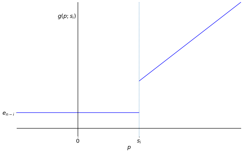The function $g(p;s_{i})$ against $p$ for $s_{i}>\tilde{e}_{n-i}$

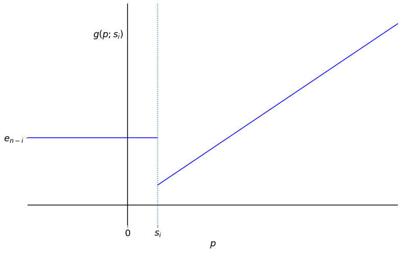The function $g(p;s_{i})$ against $p$ for $s_{i}<\tilde{e}_{n-i}$

Now it is easy to see that $\tilde{e}_{n-i}$ is the unique choice of $s_i$ which maximises $g(p;s_i)$ for every $p$. That is to say, we have:

• optimality, i.e. $g(p;\tilde{e}_{n-i})\geq g(p;s_i)$ for all $p$ and $s_{i}$
• uniqueness, i.e. if $s_i\neq\tilde{e}_{n-i}$, then there exists $p$ such that $g(p;\tilde{e}_{n-i}) > g(p;s_i)$.

With this optimal choice, the above graph looks like a ramp function, with “corner” at the point $(\tilde{e}_{n-i}, \tilde{e}_{n-i})$.

In fact, this is exactly the algebraic way of framing the argument given in Turnip Mania. For any non-optimal choice of $s_{i}\neq\tilde{e}_{n-i}$, we can find an interpretation for why this choice is sub-optimal:

Non-optimal condition	Property of $g$	Interpretation
$s_{i}<\tilde{e}_{n-i}$	$g(p;s_i)=p<\tilde{e}_{n-i}=g(p;\tilde{e}_{n-i})$ for $p\in(s_{i}, \tilde{e}_{n-i})$	Never settle for a price less than $\tilde{e}_{n-i}$, better off (in expectation) by playing on
$s_{i}>\tilde{e}_{n-i}$	$g(p;s_i)=\tilde{e}_{n-i}<p=g(p;\tilde{e}_{n-i})$ for $p\in(\tilde{e}_{n-i}, s_{i})$	Not expected to receive more than $\tilde{e}_{n-i}$ by playing on

All this is to say that we recover the key fact that

\[\tilde{s_i}=\tilde{e}_{n-i}.\]

Note: The values of the optimal thresholds are only unique under the assumption that the values of the future expectations $e_{n-i}$ occur in regions of the real line where the pdf $f_{P}$ is supported. This will be the case for all of the distributions we are considering, and is the case for any distribution where the support of $f_{P}$ is a connected interval (e.g. uniform, exponential, normal). To illustrate non-uniqueness where the support of $f_{P}$ doesn’t satisfy this criterion, consider the distribution:

\[\hat{f}_{P}(p) = \left\{\begin{matrix} \frac{3}{2} & \text{for } 0\leq p\leq \frac{1}{3},\\ \frac{3}{2} & \text{for } \frac{2}{3}\leq p\leq 1, \\ 0 & \text{otherwise.} \end{matrix}\right.\]

On the penultimate day, we should clearly take the quoted price if it exceeds the expected price of $\frac{1}{2}$; however, the threshold can take any value in the interval $\left[\frac{1}{3}, \frac{2}{3}\right]$.

All that remains is to give a first order recurrence for these optimal thresholds.

Arbitrary (non-negative) turnips: a recurrence

The derivation of the recursion relation in the uniform case in a previous section was started in a generic manner, meaning we can start from the following relation, which holds for any price distribution:

\[\begin{align} \tilde{s}_{i} =&\; \mathbb{E}(P_{i + 1}|P_{i + 1}\geq \tilde{s}_{i + 1})\mathbb{P}(P_{i + 1}\geq \tilde{s}_{i + 1}) \\[5pt] &+ \tilde{s}_{i+1}\mathbb{P}(P_{i + 1} < \tilde{s}_{i + 1}). \end{align}\]

Let $F(p)$ be the cdf of each price (with associated pdf $f_{p}(p)$), and define $\bar{F}(p)=1-F(p)$. Then, in a similar way to the uniform case, we can write the above expression as:

\[\begin{align} \tilde{s}_{i} &= \mathbb{E}(P_{i+1}|P_{i+1}\geq\tilde{s}_{i+1})\bar{F}(\tilde{s}_{i+1}) + \tilde{s}_{i+1}F(\tilde{s}_{i+1}) \\[5pt] &= \tilde{s}_{i+1} + \phi(\tilde{s}_{i+1}) \end{align}\]

where the function $\phi$ is defined (using a random variable $P$ distributed like the prices $P_{i}$) by

\[\phi(t) = (\mathbb{E}(P|P\geq t) - t)\bar{F}(t).\]

Thus, to see the behaviour of the recursion relation in the general case, it remains to better understand the function $\phi(\tilde{s}_{i+1})$.

For continuously distributed $P_i$, we have

\[\begin{align} \phi(t) &= \int_{t}^\infty pf_{p}(p)\mathrm{d}p - t\bar{F}(t) \\ &= \int_{t}^{\infty}\bar{F}(p)\mathrm{d}p \end{align}\]

where the second line can be shown to be equal by expressing $\bar{F}$ in integral form and switching the orders of integration (making use of Fubini’s theorem). We note that this does not require that the random variables are non-negative. Altogether this gives

\[\tilde{s}_{i} = \tilde{s}_{i+1} + \int_{\tilde{s}_{i+1}}^{\infty}\bar{F}(p)\mathrm{d}p. \\\]

This is as far as we can get in simplifying the recursion relation in the general case. However, there is another form we can write this in when assuming that the pdf $f_{P}(p)$ is only supported for $p\geq 0$, a reasonable assumption given that $P$ represents a price. Using integration by parts, note that

\[\int_{0}^{\infty}\bar{F}(p)\mathrm{d}p=\mu\]

where $\mu=\mathbb{E}(P)$ is the mean of the quoted prices. This allows the recurrence relation to be written using a finite integral rather than an infinite one:

\[\begin{align} \tilde{s}_{i} &= \tilde{s}_{i+1} + \int_{0}^{\infty}\bar{F}(p)\mathrm{d}p - \int_{0}^{\tilde{s}_{i+1}}\bar{F}(p)\mathrm{d}p \\ &= \mu + \int_{0}^{\tilde{s}_{i+1}}\left(1 - \bar{F}(p)\right)\mathrm{d}p \\ &= \mu + \int_{0}^{\tilde{s}_{i+1}}F(p)\mathrm{d}p. \end{align}\]

A note on our assumptions: existence of expectations

We have implicitly assumed throughout that all expectations exist. This is not an issue since the original question makes little sense unless the $P_i$ have a well defined expectation, and this is enough to ensure that all later expectations exist.

Discrete random variables

We have also assumed throughout that the random variables $P_{i}$ are continuously distributed. In the case that they are discretely distributed instead, we still have the formula for the recursion function $\phi$:

\[\phi(t) = (\mathbb{E}(P|P\geq t) - t)\bar{F}(t)\]

and from here on, similar results for the threshold recursion relation can be shown using summations instead of integrals, and the pmf rather than the pdf for the random variable $P$. As mentioned in an earlier note, the threshold will no longer be unique in this case, but there is a natural choice of unique threshold by restricting possible thresholds to values where the pmf is non-zero (i.e. prices which can actually be realised). As the specific examples of distributions for $P$ that we will be considering are all continuous, we will not give the discrete case any further attention.

Carpe rāpa!: optimality and sticking to your guns

It is high time we address one small technical question: must the optimal strategy actually be of the form we have been considering? Recall that we have thus for only considered strategies of the form:

Sell at time $i$ if $P_{i}\geq s_{i}$

That is, the price we sell at on each given day depends only upon the day itself – we do not dwell on the past and factor in the prices we’ve seen so far. Since we ought to assume that the buyer only has knowledge of past and not future prices, the most general form a strategy could take would be:

Sell at time $i$ if $P_{i}\geq s_{i}(P_1, \ldots, P_{i-1})$

where each $s_i$ is a function of the previous $i-1$ prices offered. We note that regardless of the specific distribution of the $P_i$ we will always have, for any $i$, that

\[\mathbb{E}(S) = \mathbb{E}(S|\tau < i)\mathbb{P}(\tau < i) + \mathbb{E}(S|\tau \geq i)\mathbb{P}(\tau \geq i).\]

As remarked earlier, $\mathbb{E}(S|\tau < i)$, $\mathbb{P}(\tau < i)$ and $\mathbb{P}(\tau \geq i)$ depend only upon $s_1,\ldots, s_{i-1}$, whereas $\mathbb{E}(S|\tau \geq i)$ depends upon $s_i, \ldots, s_n$. In particular, the only term that depends upon the threshold $s_i$ does not depend upon any of the earlier thresholds. Moreover, as the conditional expectation of $S$ given that $\tau\geq i$ and any such fixed specification of $P_1,\ldots, P_{i-1}$ does not depend upon the specific choice of these prices, we can maximise the expectation by choosing $s_i$ purely in terms of the later thresholds. That is to say, we can happily restrict our attention to those strategies with a fixed threshold for each day, not depending upon previous days.

Outstanding questions

Now that we’ve shown that the optimal thresholds are indeed the ‘play on’ expectations, and found a rather simple looking (albeit non-linear) first order recurrence governing these, a few questions come to mind.

Other test cases

It’s natural to wonder if there are any other reasonably natural distributions for which we can solve, exactly or approximately, the first order recurrence governing the optimal threshold.

Arbitrary turnips

On top of this, it would be great to be able to say something about the solution in general.

Next time: Asymptotic Swede

In the next post we hope to address both of these questions.

Footnotes

1 This author doesn’t know to what degree people know their models to be correct. It’s my understanding that the way the prices are generated hasn’t changed a great deal for earlier games in the series but I’m unsure if at any point people were certain of the model in the sense that they had seen the code, or whether they’re simply certain in the sense that it has been experimentally verified to some high degree of accuracy.

2 One could argue that the existence of these tools is in itself SPOILERS.

3 It is the assumption of independence that causes our model to not accurately describe the true behaviour of the turnip pricing in Animal Crossing.