Animal Crossing Turnip Market – Turnip Mania

December 30, 2020 11 minute read

This post is written in collaboration with Jack Bartley, while playing Animal Crossing New Horizons.

The Stalk Market

In the game, one of the fastest ways of earning bells (the in game currency) and pay off your mortgage to Tom Nook is through the Stalk Market; essentially, this involves speculating on the price of turnips (chosen because the Japanese word for turnip, 蕪 (kabu) is pronounced in the same way as 株 (kabu), the word for stock).

So how does it work? The way in which turnips can be used to make a profit (or loss) is as follows:

Every Sunday, a character called Daisy Mae can be found wandering around the island. She will offer to sell the player turnips at a randomly chosen (integer between 90 and 110) base price.


Daisy Mae peddling her wares

On every other day of the week, Timmy and Tommy in Nook’s Cranny will offer to buy turnips from you. They will offer two prices a day (one in the morning, one in the afternoon), which may be higher or lower than the base price that the turnips were bought for from Daisy Mae.


A thoroughly underwhelming offer from Timmy

One of the first questions we can ask is the following: if we know the distribution of prices that Timmy and Tommy offer on any particular day, what is the best way to maximise the amount received for the turnips? As is common we are interested in trying to maximise the expected profit.


Daisy Mae explains

An instructive example: Uniformly distributed quotes

The easiest distribution to consider is the uniform distribution – specifically, let’s assume that on each selling day, Timmy and Tommy offer a price that is uniformly distributed over some interval.

Let $P_{1}, …, P_{n}\sim U[0, 1]$ be iid random variables, representing the price offered at time $i=1,…,n$, and suppose that the turnips spoil before another is offered, becoming worthless (in the game, this is the time that Daisy Mae offers to sell you more turnips at a new price). Let $S$ be the price the turnips are sold to Timmy and Tommy.

Finding an optimal strategy

Consider the following strategy:

Sell at time $i$ if $P_{i}\geq s_{i}$.

Put simply, at each time $i$ there is a threshold value $s_{i}$ which represents the minimum price at which we will be prepared to sell. For example, as we need to sell the turnips before they spoil, we should accept any price at time $t=n$; in other words, an optimal strategy should have $s_{n}=0$. Under this strategy, we wish to compute the expected value of the selling price $S$; then by carefully choosing the threshold values, we can maximise the expected price we get for our turnips.

Keeping it simple

In the spirit of keeping things as simple as we can for as long as we can will first calculate this expectation in a fairly direct way. We will split the expectation up depending upon the day that the turnips are sold (using the law of total expectation).

The probability that the turnips are sold on the first day is simply the probability that $P_1\geq s_1$, that is $1-s_1$. Then, if the price is at least $s_1$, it is consequently uniformly distributed from $s_1$ to $1$, and as such its expectation is simply their average: $\frac{1}{2}(1+s_1)$. The contribution to the overall expectation is then simply the product of $1-s_1$ and $\frac{1}{2}(1+s_1)$, that is $\frac{1}{2}(1-s_1^2)$.

Similarly, the turnips are sold on the second day if both $P_1<s_1$ and $P_2\geq s_2$ which occurs with probability $s_1(1-s_2)$. Then, if the price on the second day is at least $s_2$ then it is uniformly distributed from $s_2$ to 1 and its expectation is $\frac{1}{2}(1+s_2)$. Here the contribution to the expected sale price is $\frac{1}{2}s_1(1-s_2^2)$.

Continuining in this spirit we see that the turnips are sold on the $i$th day if $P_1<s_1$, $P_2<s_2$, $\ldots$, $P_{i-1}<s_{i-1}$ and $P_i\geq s_i$. This has likelihood $s_1 s_2\cdots s_{i-1}(1-s_i)$. Then, as before, subject to having $P_i\geq s_i$ the expected price is $\frac{1}{2}(1+s_i)$ and as such the contribution to the expected sale price is $\frac{1}{2}s_1 s_2\cdots s_{i-1}(1-s_i^2)$.

Putting this all together gives the expected sale price:

\[\begin{align} \mathbb{E}(S)=&\;\frac{1}{2}(1-s_1^2)\\ +&\;\frac{1}{2}s_1(1-s_2^2)\\ +&\;\ldots\\ +&\;\frac{1}{2}s_1 s_2\cdots s_{n-2}(1-s_{n-1}^2)\\ +&\;\frac{1}{2}s_1 s_2\cdots s_{n-2}s_{n-1}(1-s_n^2). \end{align}\]

At first this looks as though it could be a little unwieldy. We notice however that $s_n$ only appears in the final term and that, fixing the other thresholds, the expectation is maximised when $s_n=0$. Let’s write $\tilde{s}_n=0$ for this optimal threshold. Now let’s revisit the expectation, leaving $\tilde{s}_n$ in place for reference:

This time we notice that the only terms featuring $s_{n-1}$ are the last two. In fact, more than this, the last two terms depend upon the earlier thresholds $s_1, s_2, \ldots, s_{n-2}$ in exactly the same way. That is, taking out a factor of $\frac{1}{2}s_1 s_2\cdots s_{n-2}$ from both the last two terms we are left with something that depends only upon $s_{n-1}$ and our optimal threshold $\tilde{s}_n$. Specifically this leaves

\[1-s_{n-1}^2+s_{n-1}(1-\tilde{s}_n^2).\]

Note that this is of the form $1-x^2+ax$ for $x=s_{n-1}$ and $a=1-\tilde{s}_n^2=1$ which is maximised when $x=\frac{1}{2}a=\frac{1}{2}$ and as such we see that $\tilde{s}_{n-1}=\frac{1}{2}$.

So far so good! Perhaps we can continue in this way and find the optimal thresholds by working backwards. Let’s next look at $s_{n-2}$. Considering again the expected sale price we have

\[\begin{align} \mathbb{E}(S)=&\;\frac{1}{2}(1-s_1^2)\\ +&\;\frac{1}{2}s_1(1-s_2^2)\\ +&\;\ldots\\ +&\;\frac{1}{2}s_1 s_2\cdots s_{n-3}(1-s_{n-2}^2)\\ +&\;\frac{1}{2}s_1 s_2\cdots s_{n-3}s_{n-2}(1-\tilde{s}_{n-1}^2)\\ +&\;\frac{1}{2}s_1 s_2\cdots s_{n-3}s_{n-2}\tilde{s}_{n-1}(1-\tilde{s}_n^2). \end{align}\]

Much as before only the last three terms feature $s_{n-2}$, and as before they depend on the earlier thresholds via the same common factor of $\frac{1}{2}s_1 s_2\cdots s_{n-3}$. Taking this factor out leaves:

\[\begin{align} &\;(1-s_{n-2}^2)\\ +&\;s_{n-2}(1-\tilde{s}_{n-1}^2)\\ +&\;s_{n-2}\tilde{s}_{n-1}(1-\tilde{s}_n^2). \end{align}\]

This is again of the form $1-x^2+ax$, with $x=s_{n-2}$ and

\[\begin{align} a&=1-\tilde{s}_{n-1}^2\\ &+\tilde{s}_{n-1}(1-\tilde{s}_n^2). \end{align}\]

But since $\tilde{s}_{n-1}=\frac{1}{2}$ we have $a=\frac{5}{4}$ and $\tilde{s}_{n-2}=\frac{5}{8}$.

Let’s now see if we can’t generalise this argument. Suppose we have already found the optimal thresholds $\tilde{s}_{i+1}, \tilde{s}_{i+2}, \ldots, \tilde{s}_n$, and wish to find the optimal threshold $\tilde{s}_i$. The expected sale price is

\[\begin{align} \mathbb{E}(S)=&\;\frac{1}{2}(1-s_1^2)\\ +&\;\frac{1}{2}s_1(1-s_2^2)\\ +&\;\ldots\\ +&\;\frac{1}{2}s_1 s_2\cdots s_{i-2}(1-s_{i-1}^2)\\ +&\;\frac{1}{2}s_1 s_2\cdots s_{i-2}s_{i-1}(1-s_i^2)\\ +&\;\frac{1}{2}s_1 s_2\cdots s_{i-2}s_{i-1}s_i(1-\tilde{s}_{i+1}^2)\\ +&\;\frac{1}{2}s_1 s_2\cdots s_{i-2}s_{i-1}s_i \tilde{s}_{i+1}(1-\tilde{s}_{i+2}^2)\\ +&\;\ldots\\ +&\;\frac{1}{2}s_1 s_2\cdots s_{i-2}s_{i-1}s_i \tilde{s}_{i+1}\cdots \tilde{s}_{n-1}(1-\tilde{s}_n^2). \end{align}\]

Now, as before, only the later terms feature $s_i$, so we can focus only on those terms. Taking the common factor of $\frac{1}{2}s_1 s_2\cdots s_{i-2}s_{i-1}$ out from those terms then leaves

\[\begin{align} &\;1-s_i^2\\ +&\;s_i(1-\tilde{s}_{i+1}^2)\\ +&\;s_i \tilde{s}_{i+1}(1-\tilde{s}_{i+2}^2)\\ +&\;\ldots\\ +&\;s_i \tilde{s}_{i+1}\cdots \tilde{s}_{n-1}(1-\tilde{s}_n^2). \end{align}\]

This is again of the form $1-x^2+ax$ where $x=s_i$ and

\[\begin{align} a=&\;1-\tilde{s}_{i+1}^2\\ +&\;\tilde{s}_{i+1}(1-\tilde{s}_{i+2}^2)\\ +&\;\ldots\\ +&\;\tilde{s}_{i+1}\cdots \tilde{s}_{n-1}(1-\tilde{s}_n^2). \end{align}\]

Therefore we obtain

\[\begin{align} \tilde{s}_i=&\;\frac{1}{2}(1-\tilde{s}_{i+1}^2)\\ +&\;\frac{1}{2}\tilde{s}_{i+1}(1-\tilde{s}_{i+2}^2)\\ +&\;\ldots\\ +&\;\frac{1}{2}\tilde{s}_{i+1}\cdots \tilde{s}_{n-1}(1-\tilde{s}_n^2). \end{align}\]

Now finally, since

\[\begin{align} \tilde{s}_{i+1}=&\;\frac{1}{2}(1-\tilde{s}_{i+2}^2)\\ +&\;\ldots\\ +&\;\frac{1}{2}\tilde{s}_{i+2}\cdots \tilde{s}_{n-1}(1-\tilde{s}_n^2). \end{align}\]

we see that

\[\begin{align} \tilde{s}_i=&\;\frac{1}{2}(1-\tilde{s}_{i+1}^2)\\ +&\;\tilde{s}_{i+1}^2\\ =&\;\frac{1}{2}(1+\tilde{s}_{i+1}^2). \end{align}\]

So we see that the optimal thresholds satisfy a reasonably simple first order backwards recursion relation

\[\tilde{s}_i=\frac{1}{2}(1+\tilde{s}_{i+1}^2).\]

The recursion relation for $\tilde{s}_{i}$

At first glance, this recurrence relation is not particular familiar; however, by performing the substitution $t_{k}=\frac{1}{2}(1-\tilde{s}_{n-k})$, we obtain

\[t_{i+1} = t_{i}(1-t_{i}), \quad t_{0} = \frac{1}{2}\]

Hopefully, this rings some bells! It should be familiar to any first year mathematics undergraduates as a special case of the logistic map, the general form of which looks like:

\[t_{i+1} = r t_{i}(1-t_{i}).\]

In our case, the reproductive parameter $r=1$, and the initial value $t_{0}=\frac{1}{2}$. This recurrence relation is often first encountered when considering the dynamics of a population of animals living in an environment with limited resources, and is usually used as an introduction to chaos theory. In this context, it suffices to say that for this choice of reproductive parameter, $t_{i}$ is decreasing as $i$ increases, and gets arbitrarily close to $0$ for sufficiently large $i$. This is as expected from our problem - if there are a large number of times over which prices can be tracked, then over the first few times the price needs to be very high in order to tempt the seller.


One of the many exciting plots you get to see when studying the logistic function, showing the convergence value as $i\rightarrow\infty$ for various values of $r$, the reproductive parameter.

Uniformly distributed quotes: a numerical solution

To compute the actual threshold values and expectations, we turn to some simple Python functions; the optimal thresholds are computed using the recursion relation, and the expectation is then computed directly using these threshold values:

def compute_exp(s):
    """Expected value of the strategy.
    
    Computes the expected value of the strategy, defined by
    the vector of strategy thresholds.

    Args:
        s (numpy.ndarray): Vector of threshold values.

    Returns:
        expectation (float): Expected value of the strategy
    """
    expectation = 0
    for i in range(len(s)):
        expectation += 0.5*(1 - s[i]**2)*np.prod(s[:i])
    return expectation

def strat_thresholds(n):
    """Strategy thresholds for uniformly distributed prices.
    
    Computes the threshold values of the optimal strategy, when 
    prices are drawn from an uniform distribution.

    Args:
        n (int): Number of times over which prices are offered.

    Returns:
        s (numpy.ndarray): vector of optimal strategy values.
    """
    s = np.zeros(n)
    
    for i in range(n-1):
        s[i+1] = 0.5*(1 + s[i]**2)
    s = s[::-1]
    
    return s

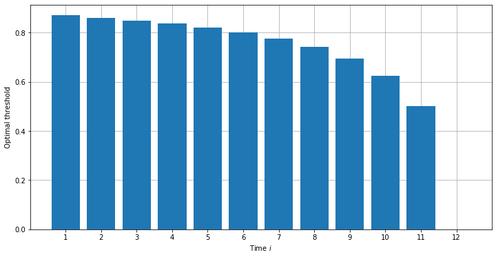
For example, if prices are provided over 12 times (the number of opportunities allowed in Animal Crossing - twice a day, Monday to Saturday), the threshold at the first time is about 0.88, decreasing to 0 at the last time when any price has to be taken:

thresholds = strat_thresholds(n=12)
expectation = compute_exp(thresholds)
print(f'Thresholds are: ')
for time, threshold in enumerate(thresholds):
    print(f'Time {time+1}: {threshold}')
print(f'giving an expected sold price of {expectation}')

Thresholds are: 
Time 1: 0.8707450655319368
Time 2: 0.861098212205712
Time 3: 0.8498214073624081
Time 4: 0.8364465402671089
Time 5: 0.8203006037631678
Time 6: 0.800375666500635
Time 7: 0.7750815008766949
Time 8: 0.741729736328125
Time 9: 0.6953125
Time 10: 0.625
Time 11: 0.5
Time 12: 0.0
giving an expected sold price of 0.8790984845741084

These optimal thresholds are easier to visualise when plotted on a graph, showing the threshold for each day of the 12-period run:


The optimal thresholds for each day of a 12-period run

It is also easy to check that as the number of times increases, the expected price that the seller can get increases, due to the ability they have to hold out for a randomly occurring larger price:

print('Expectation for n times:')
for time in range(1, 21):
    thresholds = strat_thresholds(n=time)
    print(f'{time} times: {compute_exp(thresholds)}')

Expectation for n times:
times: 0.5
times: 0.625
times: 0.6953125
times: 0.741729736328125
times: 0.7750815008766949
times: 0.800375666500635
times: 0.8203006037631679
times: 0.8364465402671089
times: 0.8498214073624082
times: 0.8610982122057119
times: 0.8707450655319368
times: 0.8790984845741084
times: 0.886407072790247
times: 0.892858749346287
times: 0.8985983731421079
times: 0.9037395181068213
times: 0.908372558293975
times: 0.9125703523307703
times: 0.9163923239765532
times: 0.919887445721574

Thresholds and expectations

It’s interesting to observe that there appears to be a relationship between the expected values and the thresholds themselves. Indeed, it appears that the optimal threshold at time $n-i$, that is $\tilde{s}_{n-i}$, is the same as the expected value (arising from the optimal strategy of this type) for the game in which only the first $i$ prices are offered, or equivalently, because of the backwards recursion relating the optimal thresholds, the expected sale price if the player rejects the price at time $n-i$ and instead plays on.

For clarity we write $\tilde{e}_n$ for $\mathbb{E}(S)$, the expected sale price for the game played over $n$ days, when following the optimal strategy of the type discussed above. Then the relationship can be stated as

\[\tilde{s}_{n-i}=\tilde{e}_i.\]

With hindsight this is not exactly surprising. We definitely shouldn’t at any point settle for a lower price than we would expect were we to play on. That is to say, we should have $\tilde{s}_{n-i}\geq\tilde{e}_i$.

In the other direction, were we to hold out for a price strictly greater than what would would achieve in expectation were we to carry on (that is, if $\tilde{s}_{n-i}>\tilde{e}_i$), then we would, informally speaking, be throwing away perfectly good prices in favour of the lower prices that we would expect in playing on.

We will revisit this a little more formally in a later post.

Outstanding questions

Isabelle thinking

After a bit of playing around with the uniform case we’ve managed to find first order recurrence describing the optimal threshold values for a strategy of this sort. This begs a few natural questions.

Seize the day!

In the above we only considered strategies of the form:

Sell at time $i$ if $P_{i}\geq s_{i}$

That is to say, the price we would settle for on each day depended only upon the day itself and not upon the prices we had seen so far. As we tacitly assume that the buyer only has knowledge of past and not future prices, a generic strategy would be of the form:

Sell at time $i$ if $P_{i}\geq s_{i}(P_1, \ldots, P_{i-1})$

where here $s_i$ is now a function of $i-1$ variables. Can we convince ourselves that optimal strategies must be of the former type?

Solving the recurrence

Having found the recurrence governing the optimal thresholds, while it may not be possible to find an exact formula for them it would be nice to be able to say something more about the solutions. Perhaps we could say something about their asymptotics?

Flying the nest

Now that we’ve cut our teeth on this simple case, we would like to say something about other distributions. In particular, can we find a simple recurrence governing the thresholds of an optimal strategy? Can we show that it is always the case the these optimal thresholds are the expected returns if we choose to play on, as discussed earlier?

Next time: Non-uniform Turnips

In the next post we will give an answer to each of the questions posed above.

Isabelle thinking

Share on

Twitter Facebook LinkedIn

Michael Cole

Jack Bartley